A Study on Visual Complexity
Table of Contents
- Introduction
- Explaining Visual Complexity using Deep Segmentation Models
- Multi-Scale Sobel Gradient
- Multi-Scale Unique Color
- Improving Predictions with MSG and MUC
- Familiarity Bias and Surprise: A Novel Dimension in Complexity Assessment
- Conclusion
Introduction
Have you ever wondered why some images feel more complex than others? What makes a Jackson Pollock painting seem more visually complex than a Mondrian? Or why a bustling city street appears more complex than an empty highway?
Visual complexity is a fundamental aspect of how we perceive images, influencing everything from user interface design to art appreciation. While we intuitively understand when something looks “complex”, quantifying this perception has proven challenging for researchers.
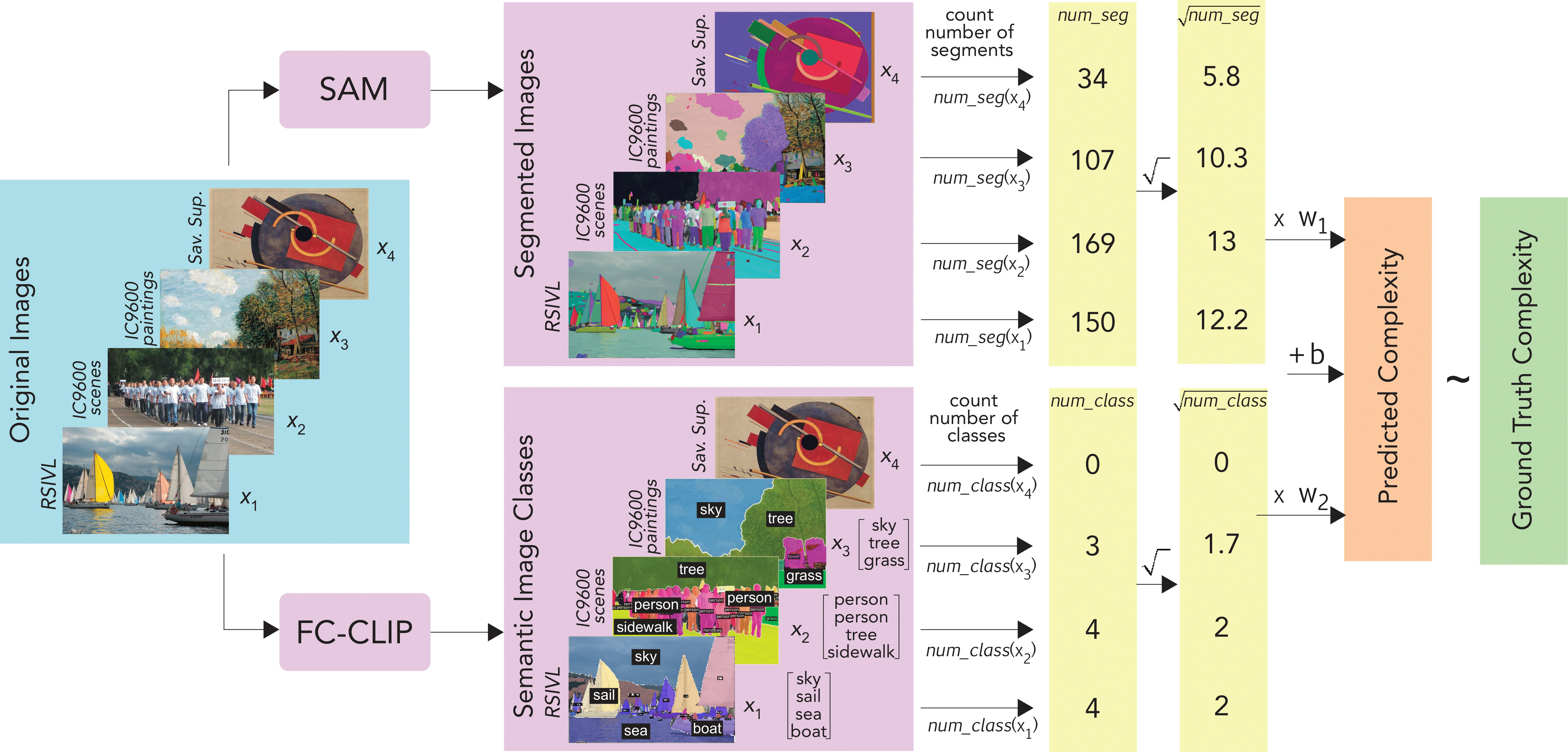
Recent work by Shen et al. (2024) made significant progress using a surprisingly simple approach. They found that just two features extracted from deep neural networks—the number of segments detected by SAM (Segment Anything Model) and the number of semantic classes identified by FC-CLIP—could explain much of human complexity judgments across diverse image datasets.
But is that all there is to visual complexity? In this post, I’ll share our recent findings that go beyond this baseline model to uncover key dimensions that influence how we perceive the complexity of images.
Explaining Visual Complexity using Deep Segmentation Models
Let’s start with a quick recap of the baseline approach. The previous model took a middle ground between handcrafted features and deep neural networks by using:
- SAM (Segment Anything Model) to detect segments at multiple spatial granularities
- FC-CLIP to identify semantic class instances in images
From these models, they extracted just two key features:
num_seg: The total number of segments detected by SAMnum_class: The number of class instances identified by FC-CLIP
After applying a square-root transformation to these features, they combined them in a simple linear regression model to predict perceived complexity.

This approach maintained interpretability while utilizing the power of modern foundation models. However, the authors acknowledged a limitation: the model struggled with images containing specific structural patterns, such as symmetries or repetitive elements.
Multi-Scale Sobel Gradient
To address the structural aspect of visual complexity, we introduced a novel feature called Multi-Scale Sobel Gradient (MSG).
The key insight here is that the human visual system processes structure at multiple scales simultaneously. When we look at an image, we perceive both fine details and larger structural elements. MSG captures this by analyzing intensity gradients at different scales.
Here’s how it works:
- We normalize the RGB image to the [0,1] range
- Define multiple scales (1, 2, 4, 8) with corresponding weights (0.4, 0.3, 0.2, 0.1)
- For each scale:
- Resize the image
- Apply Sobel operators to detect horizontal and vertical gradients in each RGB channel
- Calculate gradient magnitude
- Weight this average by the corresponding scale weight
- Sum the weighted gradient magnitudes to produce the final MSG score
MSG applies the Sobel operator across multiple resolutions to RGB images, functioning as an asymmetry detector within \(k \times k\) patches, where \(k\) represents the kernel size. For symmetric patches, the left and right columns (or rows in horizontal application) of the kernel counterbalance each other, resulting in lower MSG values. Consequently, images exhibiting greater patch-level symmetry produce smaller MSG measurements.
def calculate_msg(img):
    img = img / 255.0  # Normalize image

    scales = [1, 2, 4, 8]
    weights = [0.4, 0.3, 0.2, 0.1]

    msg_score = 0
    for s, w in zip(scales, weights):
        scaled = resize(img, (height//s, width//s))  # Resize image

        channel_grads = []
        for c in range(3):  # RGB channels
            gx = sobel(scaled[:,:,c], dx=1, dy=0) # Apply Sobel operators
            gy = sobel(scaled[:,:,c], dx=0, dy=1)

            mag = np.sqrt(gx**2 + gy**2)    # Calculate gradient magnitude
            channel_grads.append(np.mean(mag))

        # Average across channels and weight
        msg_score += w * np.mean(channel_grads)
    return msg_score
Note that the Sobel operator is typically applied to grayscale images, but we found in ablations that the grayscale version of the algorithm (which first converts the colored images to grayscale) did not perform as well. Hence we use the color version of the algorithm for the rest of our study.
Multi-Scale Unique Color
Color diversity also plays a significant role in visual complexity, particularly in artistic and designed images. To capture this dimension, we developed Multi-Scale Unique Color (MUC), which counts unique colors at multiple scales and color resolutions.
MUC works as follows:
- Define multiple scales (1, 2, 4, 8) with weights (0.4, 0.3, 0.2, 0.1)
- For each scale:
- Resize the image
- Quantize colors by reducing bit precision
- Count unique colors in the resized, quantized image
- Weight this count by the scale weight
- Sum the weighted color counts
def calculate_muc(img, bits_per_channel=7):
    scales = [1, 2, 4, 8]
    weights = [0.4, 0.3, 0.2, 0.1]

    muc_score = 0

    for s, w in zip(scales, weights):
        # Resize image to analyze color at different spatial resolutions
        h, w_img, _ = img.shape
        resized = resize(img, (h//s, w_img//s))

        shift = 8 - bits_per_channel  # Calculate bit shift
        quantized = (resized >> shift) << shift  # Reduce precision

        flat = quantized.reshape(-1, 3)  # Flatten to pixel array
        # Create single integer index for each RGB color
        indices = (flat[:, 0] << 16) | (flat[:, 1] << 8) | flat[:, 2]

        unique_colors = len(np.unique(indices))  # Count unique colors
        muc_score += w * unique_colors # Weight by scale weight and add to total

    return muc_score
This approach provides a robust measure of chromatic complexity that aligns well with human perception, especially for artistic images.
Improving Predictions with MSG and MUC
Our experiments across 16 datasets show that adding MSG and MUC to the baseline model significantly improves performance. Here are some highlights:
- On the VISC dataset of natural images, adding MSG improved correlation from 0.56 to 0.68
- For the IC9 Architecture dataset, MSG increased correlation by 0.10, increasing it from 0.66 to 0.76.
- On the Savoias Art dataset, MUC boosted correlation from 0.73 to 0.81.
- For Savoias Suprematism (abstract art), MUC improved performance from 0.89 to 0.94.
Most impressively, combining both MSG and MUC led to enormous gains on certain datasets:
- Savoias Interior Design: from 0.61 to 0.87 (+0.26).
- IC9 Abstract: from 0.66 to 0.83 (+0.17).
Comparison with Patch-Based Symmetry and Edge Density
We also compared MSG against two common structural features:
- Patch-based symmetry (a measure of how symmetrical small image patches are)
- Canny edge density (a standard metric for image complexity)
We run permutation tests to detect any statistical superiority between the methods. Our comprehensive comparison shows that MSG demonstrates superior performance with a win/loss/tie record of 5/2/9 against Canny edge density (where the remaining 9 datasets showed no statistically significant difference) and 7/1/8 against patch symmetry. Our ablations confirm that MSG is currently the most performant structural feature for predicting complexity across diverse image datasets.
Single vs. Multi-Scale
An important question was whether the multi-scale approach actually improved performance. Our ablation studies confirmed this:
- Multi-scale MSG outperformed single-scale MSG on 6 datasets (6/2/8)
- Multi-scale MUC outperformed single-scale MUC on 5 datasets (5/1/10)
This validates our hypothesis that analyzing images at multiple scales better aligns with how the human visual system processes complexity.
Familiarity Bias and Surprise: A Novel Dimension in Complexity Assessment
While improving our features for structure and color, we discovered another dimension of visual complexity: surprise.
Previous research by Forsythe et al. showed that humans perceive familiar images as less complex than unfamiliar ones, even when their objective complexity is the same. This “familiarity bias” suggests that our perception of complexity isn’t just about what’s in the image, but also how our brain processes it based on prior experience.
We decided to test whether the opposite of familiarity—surprise—contributes to perceived visual complexity.
Experimental Setup
To investigate this, we created a novel dataset called Surprising Visual Genome (SVG). This dataset contains:
- 100 highly surprising images
- 100 randomly sampled (less surprising) images from Visual Genome
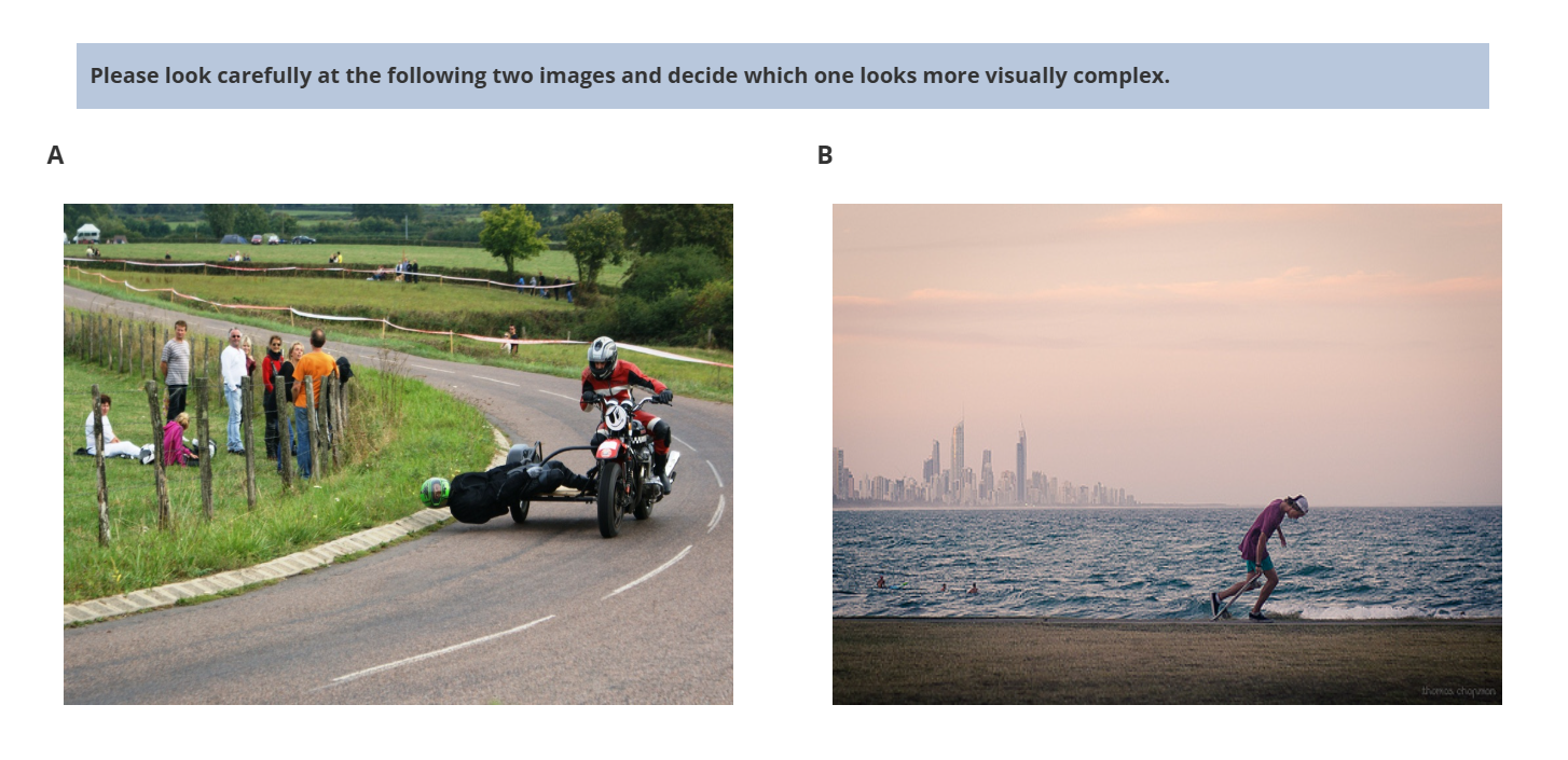
We collected human complexity ratings through an online experiment where participants compared image pairs and selected the more complex one. Using the Bradley-Terry algorithm, we converted these pairwise comparisons into scalar complexity ratings.

One fascinating insight came from participants’ descriptions of how they judged complexity. Many mentioned that “unusual,” “surprising,” or “weird” content made images seem more complex:
| Participant Responses |
|---|
| “How many different elements there were in each photo and how surprising or unusual the images were.” |
| “The weird or uncanny images appeared quite complex to me, most of the landscape shots or regular street/traffic scenes didn’t strike me as complex.” |
| “I think it was a mix of structure of the image and the elements within it—the more unusual or juxtaposed the mix, the more complex it appeared to me.” |
Generating Surprise Scores
To quantify surprise, we used a large language model (Gemini-Flash-1.5) with Chain-of-Thought prompting. We asked the model to:
Prompt: Zero-shot-CoT
Q: Step by step, explain why this image is surprising or not. Consider factors like rare events, or unexpected content. Be precise in your reasoning. Then, on a precise scale from 0 to 100, rate the surprisal of this image.
Provide your reasoning and numeric rating as follows:
Reasoning: [your explanation]
Rating: <<number>>

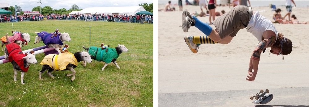
Here are the surprise evaluations provided by the LLM for two images from SVG:
Example LLM Surprise Evaluations
Surprise score: 85
Reasoning: The image depicts sheep dressed in jockey silks and participating in a race. This is surprising because it is not a typical activity for sheep. The use of animals in a human sport is unexpected and humorous. The precise arrangement of the sheep with racing attire transforms an ordinary farm animal into an amusing spectacle.
Surprise score: 85
Reasoning: The image depicts a skateboarder performing an unexpected maneuver on a beach, resulting in an unusual pose mid-air. The rarity stems from the seemingly uncontrolled backflip and the unusual beach setting for such a stunt. His body is completely inverted with the skateboard detached beneath him, heightening the surprisingness of the moment.
This approach provided not just numerical scores but also interpretable explanations for why an image might be perceived as surprising.
Results
| Model/Dataset | VISC | IC9. Arch. | Sav. Art | Sav. Sup. | Sav. Int. | IC9. Abstract | SVG |
|---|---|---|---|---|---|---|---|
| Handcrafted features | |||||||
| Corchs 1 (10 features) | 0.62 | 0.66 | 0.68 | 0.80 | 0.85 | 0.74 | 0.73 |
| Kyle-Davidson 1 (2 features) | 0.60 | 0.54 | 0.55 | 0.79 | 0.74 | 0.69 | 0.70 |
| CNNs | |||||||
| Saraee (transfer) | 0.58 | 0.59 | 0.55 | 0.72 | 0.75 | 0.67 | 0.72 |
| Feng (supervised) | 0.72 | 0.92* | 0.81 | 0.84 | 0.89 | 0.94* | 0.83 |
| Previous simple model | |||||||
| √num_seg + √num_class | 0.56 | 0.66 | 0.73 | 0.89 | 0.61 | 0.66 | 0.78 |
| Visual features | |||||||
| MSG + MUC | 0.60 | 0.65 | 0.64 | 0.91 | 0.84 | 0.76 | 0.72 |
| Baseline + visual features | |||||||
| √num_seg + √num_class + MSG | 0.68 (+0.13) | 0.76 (+0.10) | 0.75 | 0.90 | 0.79 | 0.79 | 0.78 |
| √num_seg + √num_class + MUC | 0.62 | 0.71 | 0.81 (+0.08) | 0.94 (+0.05) | 0.80 | 0.76 | 0.79 |
| √num_seg + √num_class + MSG + MUC | 0.68 | 0.77 | 0.81 | 0.94 | 0.87 (+0.26) | 0.83 (+0.17) | 0.79 |
| Baseline + semantic feature | |||||||
| √num_seg + √num_class + Surprise | 0.60 | 0.67 | 0.74 | 0.89 | 0.60 | 0.67 | 0.83 (+0.05) |
| Baseline + all features | |||||||
| √num_seg + √num_class + MSG + MUC + Surprise | 0.71 (+0.16) | 0.78 (+0.12) | 0.81 (+0.08) | 0.94 (+0.05) | 0.87 (+0.26) | 0.84 (+0.18) | 0.85 (+0.07) |
* Results on test set
Note: Bold indicates the best model for each dataset. Values in parentheses show improvement over the baseline model.
The results were striking. Adding surprise scores to our model:
- Improved correlation on the SVG dataset from 0.78 to 0.83
- Combined with MSG and MUC, reached a correlation of 0.85
More importantly, surprise scores showed a correlation of 0.48 with complexity even after controlling for the number of segments and objects. This confirms that surprise captures a unique dimension of complexity not explained by visual features alone.
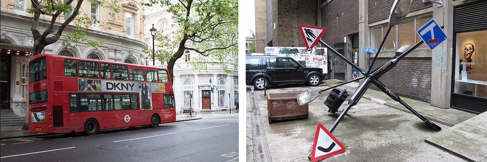
Consider these two images:

We present a case where both images share similar visual features:
| Feature | Left Image | Right Image |
|---|---|---|
| # of SAM segmentations | 191 | 172 |
| # of FC-CLIP classes | 9 | 9 |
| MSG | 59 | 56 |
| MUC | 922 | 820 |
| Surprise | 25 | 85 |
The right image, with slightly lower feature values, was initially predicted to have lower complexity. The left image received a complexity score of 60, while the right received 55. However, the element of surprise shifts the outcome, with improved predictions at 52 (72) compared to ground truth values of 25 (74). Despite their similarity, humans may perceive the second image as more complex possibly due to its unusual composition, where multiple traffic signs are clustered together.
Despite having similar visual features (segmentations, classes, gradient, color), humans perceived the right image (with multiple traffic signs clustered together) as more complex. Our model initially predicted similar complexity for both, but after adding surprise scores, it correctly distinguished between them.
Conclusion
Our research shows that visual complexity goes beyond counting objects or segments in an image. Structure (captured by MSG), color diversity (captured by MUC), and cognitive factors like surprise all contribute to how we perceive complexity.
The next time you look at an image and think “that’s complex,” remember that your brain is processing multiple dimensions of complexity—from the number of objects to the arrangement of edges, from color diversity to how surprising the content is.
This research builds upon previous work by Shen et al. (2024) on visual complexity and introduces new features and datasets for improved complexity prediction. The full paper and code are available at our GitHub repository.